bsmedit -- C/C++/SystemC Visualizer (ver 3.2.11)

1 What is bsmedit

bsmedit is a C++/SystemC Visualizer. Long time ago, when I first used the Systemc library to simulate some communication algorithms, I was quickly bored with the following debugging procedure:

update the source code;
re-compile the program;
check the results.

And occasionally, I would need to add some debugging code. For example, printing some value (e.g., printf) to the terminal or dumping the data to a file, so that I can use other tools (e.g., Matlab) to visualize and analyze it.

bsmedit aims to simplify this procedure. With bsmedit, we can

control C/C++/SystemC simulation
monitor/visualize signals in real-time
visualize VCD (value change dump) files
visualize ulog files
...

2 Get started

bsmedit can be installed with pip

$ pip install bsmedit

You can also clone the repository and run

$ cd bsmedit
$ pip install -e .

2.1 Create a SystemC simulation

To use bsmedit, the first step is to build a simulation. In the following example, we will create a dummy SystemC simulation that outputs a synchronized $\sin$ and $\cos$ waveforms.

Create a simulation project. You can use your preferred platform and compiler.
Add SystemC support to your project. To make the simulation work with bsmedit, you need a modified SystemC, which can be got here, all the branches started with bsm_ are supported by bsmedit. Currently it supports the following SystemC releases
- 3.0.0_pub_rev_20231129
- 2.3.4
- 2.3.3
- 2.3.2
- 2.3.1a
Please refer to the file INSTALL in the SystemC package about how to add SystemC support to your project.

Implement the simulation.

Create a top level SystemC module top, which may look like
```
#ifndef TOP_H_
#define TOP_H_

#include "systemc.h"

class top : public sc_module {
 public:
    SC_HAS_PROCESS(top);
    top(sc_module_name name_):
    sc_module(name_)
        , m_phase(0.0)
        , clock("CLOCK", 10, 0.5, 0.0)
        , sig_sin("sig_sin")
        , sig_cos("sig_cos")
        , sig_steps("sig_steps", 256) {
        SC_METHOD(Action);
        sensitive_pos << clock;
    }
    virtual ~top();

 private:
    void Action();

 private:
    double m_phase;
    // signal
    sc_clock clock;
    sc_signal<double> sig_sin;
    sc_signal<double> sig_cos;
    sc_signal<int> sig_steps;
};

#endif  // #ifndef TOP_H_
```
The top module is derived from sc_module. It defines several signals used in the module
- clock: the module is triggered by the positive edge of the clock, whose period is $10ns$ with 50% duty cycle. One thing to notice is that the signal clock is given a name CLOCK. bsmedit will use this name to have access to this signal. At shown in the example, the name of the signal (i.e., CLOCK) may not be same as the variable name (i.e., clock), although in practice they are often same for convenience.
- sig_sin: the signal for the sine waveform, whose name is sig_sin.
- sig_cos: the signal for the cos waveform, whose name is sig_cos.
- sig_steps: the phase step for each clock, which is increased by $\frac{\pi}{\textrm{sig_steps}}$. The phase is initialized to be zero.
The module also defines a process method (i.e., Action). It is triggered at each rising edge of clock (also called positive edge), where all calculations are conducted.

The top.cpp may look like

#include <math.h>
#include "top.h"
#ifndef M_PI
#define M_PI       3.14159265358979323846
#endif

top::~top() {
}

void top::Action() {
    sig_sin.write(sin(m_phase));
    sig_cos.write(cos(m_phase));
    int steps = sig_steps.read();
    if (steps < 256) {
        steps = 256;
        sig_steps.write(256);
    }
    m_phase = m_phase + M_PI / steps;
    if (m_phase > 2 * M_PI) m_phase -= 2 * M_PI;
}

In the process method (Action), we simply update the sin/cos signals based on the current phase. Then, update the phase for the next step. In this demo, the maximum step is assumed to be $\frac{\pi}{256}$.

The main function may look like
```
#include "systemc.h"
extern "C" {
#include "sysc/bsm/bsm.h"
}
#include "top.h"

// define the interfaces to bsmedit
BSMEDIT_IMPLEMENT_MODULE(top, "top");
```
Besides the SystemC library, it also needs to include the bsm.h/cpp in the project. They define interfaces to communicate with bsmedit
- BSMEDIT_IMPLEMENT_MODULE(top, "top") creates the top level module from class top with name "top".
We will discuss the macro in detail in the following sections.

The makefile may look like

SYSC_DIR =$(SYSTEMC_ROOT)/include
SYSC_LIB =$(SYSTEMC_ROOT)/lib-macosx64/libsystemc.a

CC = g++ -std=c++17
CFLAGS = -Wall -fexceptions -g -W -fPIC -DSC_INCLUDE_FX -DPURIFY -D_USRDLL -DBSM_DLL_SIM
LDFLAGS = -Wl,-U,_sc_main,-U,___sanitizer_start_switch_fiber,-U,___sanitizer_finish_switch_fiber

DEPS = top.h
ODIR=obj
OBJ = main.o top.o
OBJS = $(patsubst %,$(ODIR)/%,$(OBJ))

libstart: $(OBJS) $(SYSC_LIB)
    g++ -shared  $(LDFLAGS) $^ -o $@.so

$(ODIR)/%.o: %.cpp $(DEPS)
    ${CC} $(CFLAGS) -I$(SYSC_DIR) -c $< -o $@

$(OBJS): | $(ODIR)

$(ODIR):
    mkdir -p $(ODIR)

.PHONY: clean

clean:
    rm -f $(ODIR)/*.o *.so
    rm -r $(ODIR)

When compile the simulation, the compiler setting (e.g., CC in the above makefile) needs to be same as the one used to compile the SystemC library.

Compile the project to get simulation (e.g., start.dll)

The demo project can be download here.

2.2 Open with bsmedit

Make sure your simulation architecture match with python. For example, if your simulation is x64, you should also install the x64 version python. Otherwise, bsmedit will fail to load the simulation.

Start bsmedit by

$ bsmedit

and create the simulation¹ from the menu

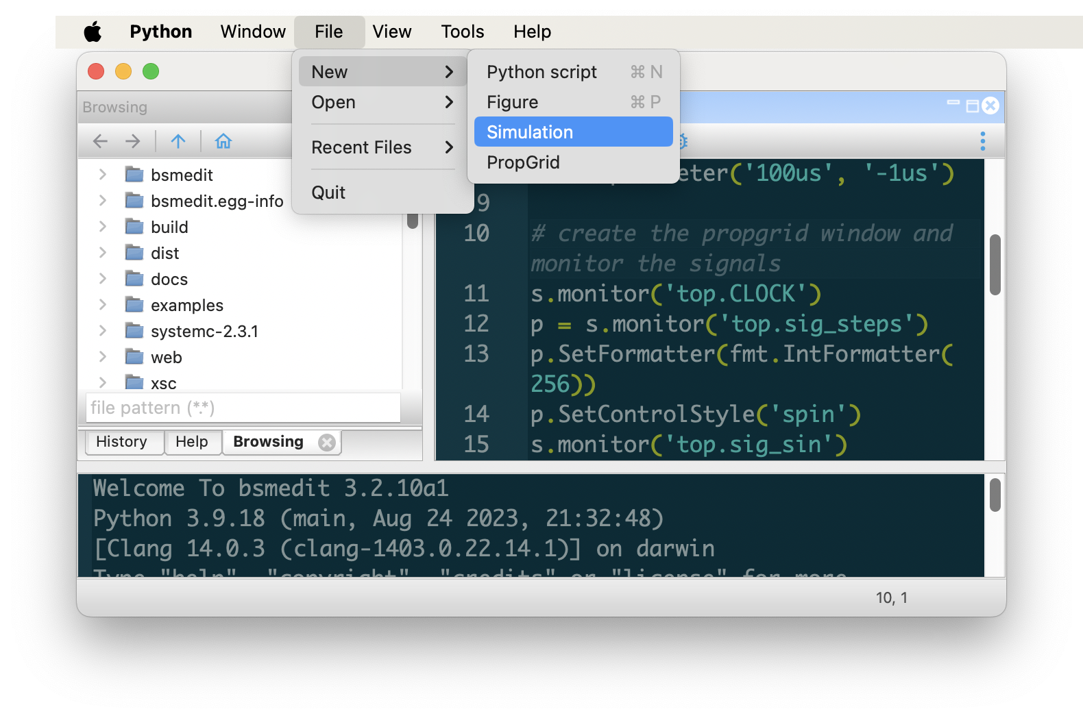
It will show a open file dialog to select the simulation library (e.g. libstart.so, start.dll ). Then bsmedit will load the simulation.

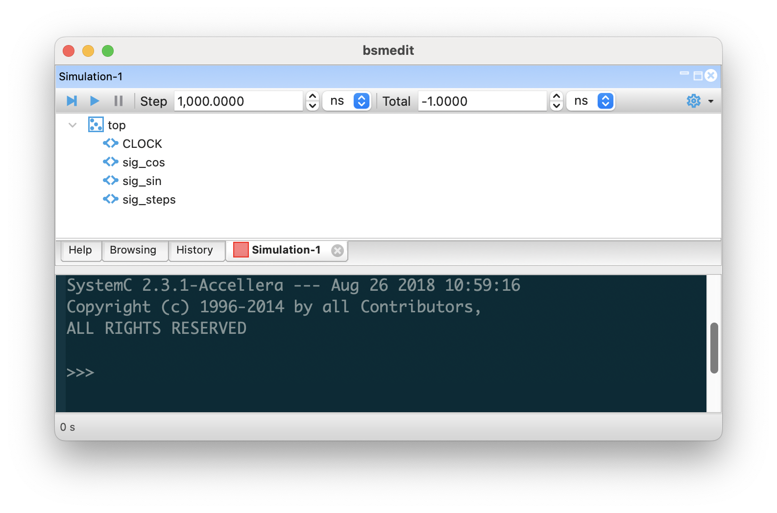
The main window consists of 4 sections, from top to bottom:

Simulation control toolbar. From left to right:
- step: run simulation in one step. You can arbitrarily define step duration. As we will show shortly, it is different from the delta cycle concept in SystemC simulation.
- run: run simulation until it is paused or total simulation duration is reached.
- pause: pause simulation.
- step duration: the duration of each simulation step. At the end of each simulation step, bsmedit will retrieve the data from the simulation and update the GUI (e.g., the time-stamp).
- step unit: the time unit of each simulation step.
- total duration: the total simulation duration. bsmedit will pause the simulation if the current simulation time exceeds the total simulation time. -1 to run simulation infinitely.
- total unit: the time unit of the total simulation duration.
Simulation objects². This window lists all objects defined in the simulation. As shown in figure above, the simulation has one top module (i.e., top) and 4 signals: CLOCK, sig_cos, sig_sin, and sig_steps. The tree hierarchy represents their structure in the simulation.
Console window. It is used to execute commands and show outputs.
Statusbar.

To run the simulation, click the step or run button. The simulation will proceed until you pause it or the total simulation duration is reached. The current simulation time is shown in the status bar.

It is not very useful if bsmedit can only control the simulation running. bsmedit also allows you to monitor the signal values in real-time: select the signal to be monitored, and right click on it

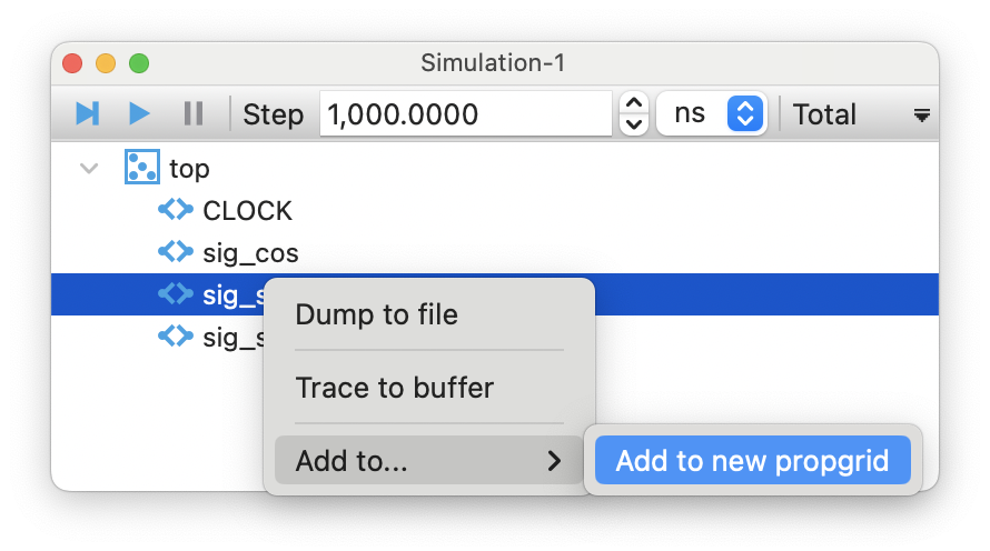
bsmedit will create a propgrid window and add the selected signals to it.

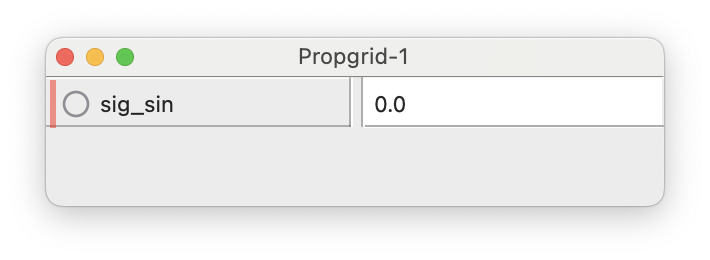
Click the run button to start the simulation. The signal value will be updated automatically.

You can also modify the signal values, for example, by typing the following commands in the console window

>>> # get the simulation handle
>>> s = simulation(1)
>>> # set the number of steps
>>> s['top.sig_steps'] = 8192

The first command gets the handle of the simulation. Then, the second command sets the value of signal top.sig_steps to 8192.

You can also plot the trace to see the signal trend,

>>> # trace the cos waveform to a buffer with size 4096
>>> s.trace_buf('top.sig_cos', 4096)
>>> # trace the sine waveform to a buffer with size 4096 too
>>> s.trace_buf('top.sig_sin', 4096)
>>> # plot the trace
>>> plot_trace('top.sig_cos', 'top.sig_sin', relim=False)
>>> xlim([-1,1])
>>> ylim([-1,1])

The first command tells bsmedit to start tracing the signal top.sig_cos; and the buffer length is 4096. In other words, its latest 4096 values will be stored in a numpy array. Similarly, the second command traces the signal top.sig_sin. The third command creates a figure to plot top.sig_cos as $x$ axis value and top.sig_sin as $y$ axis. The last two lines set the limits of $x$ axis and $y$ axis, respectively. The created figure looks like

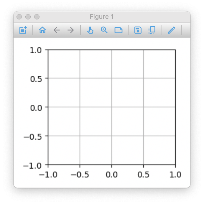
It does not really show anything, since we just create the buffer and it has not be filled with signal values yet. When you run the simulation, the buffer will be filled and the plot will be updated accordingly

You can following the above steps to start the simulation and monitor the signals each time. However, it is too tedious to repeat each step again and again. In bsmedit, you can write a python script to do all the steps. The script may look like

from bsmedit.bsm.pysim import *
from propgrid import formatters as fmt
# create a simulation
s = simulation(None, './examples/start/libstart.so')

assert s.is_valid(), "Failed to load simulation"
# set the simulation parameters: step = 100us, run infinitely
s.set_parameter('100us', '-1us')

# create the propgrid window and monitor the signals
s.monitor('top.CLOCK')
p = s.monitor('top.sig_steps')
p.SetFormatter(fmt.IntFormatter(min_value=256))
p.SetControlStyle('Spin')
s.monitor('top.sig_sin')
s.monitor('top.sig_cos')

s.write({'top.sig_steps': 2**16})
# dump the signal value to a numpy array
s.trace_buf('top.sig_cos', 2**14)
s.trace_buf('top.sig_sin', 2**14)

plot_trace('top.sig_cos', 'top.sig_sin', relim=False)
xlim([-1, 1])
ylim([-1, 1])
grid(ls='dotted')
s.run(more='1000us')
s.wait_until_simulation_paused()

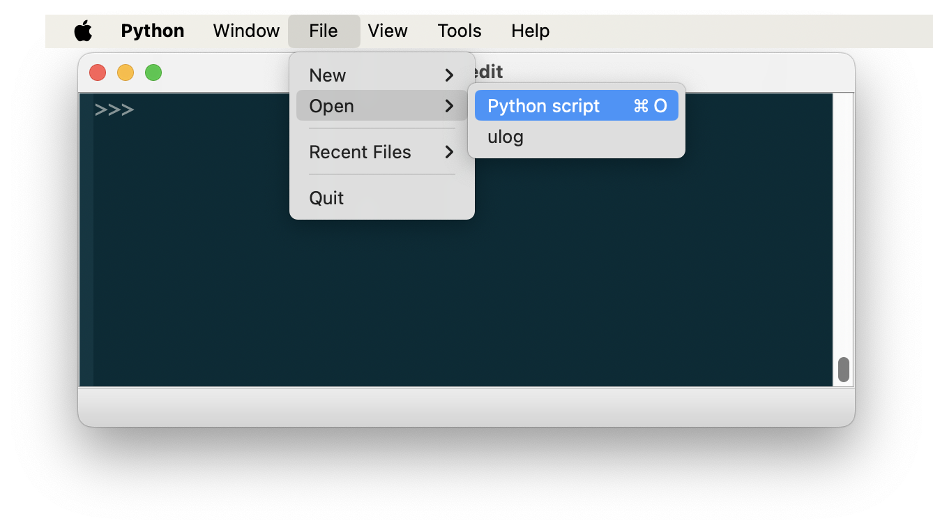
Save the script to a file (e.g., start.py). Then, it can be opened in bsmedit

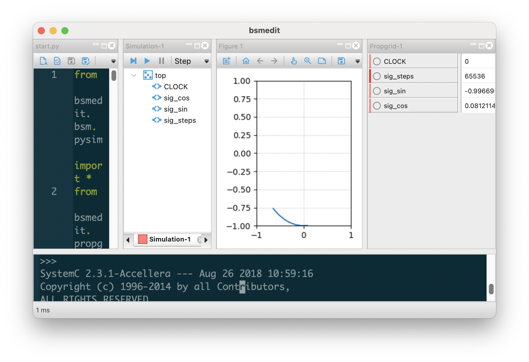
And it will look like the one shown in the following image. Click the Execute the script button to run the script

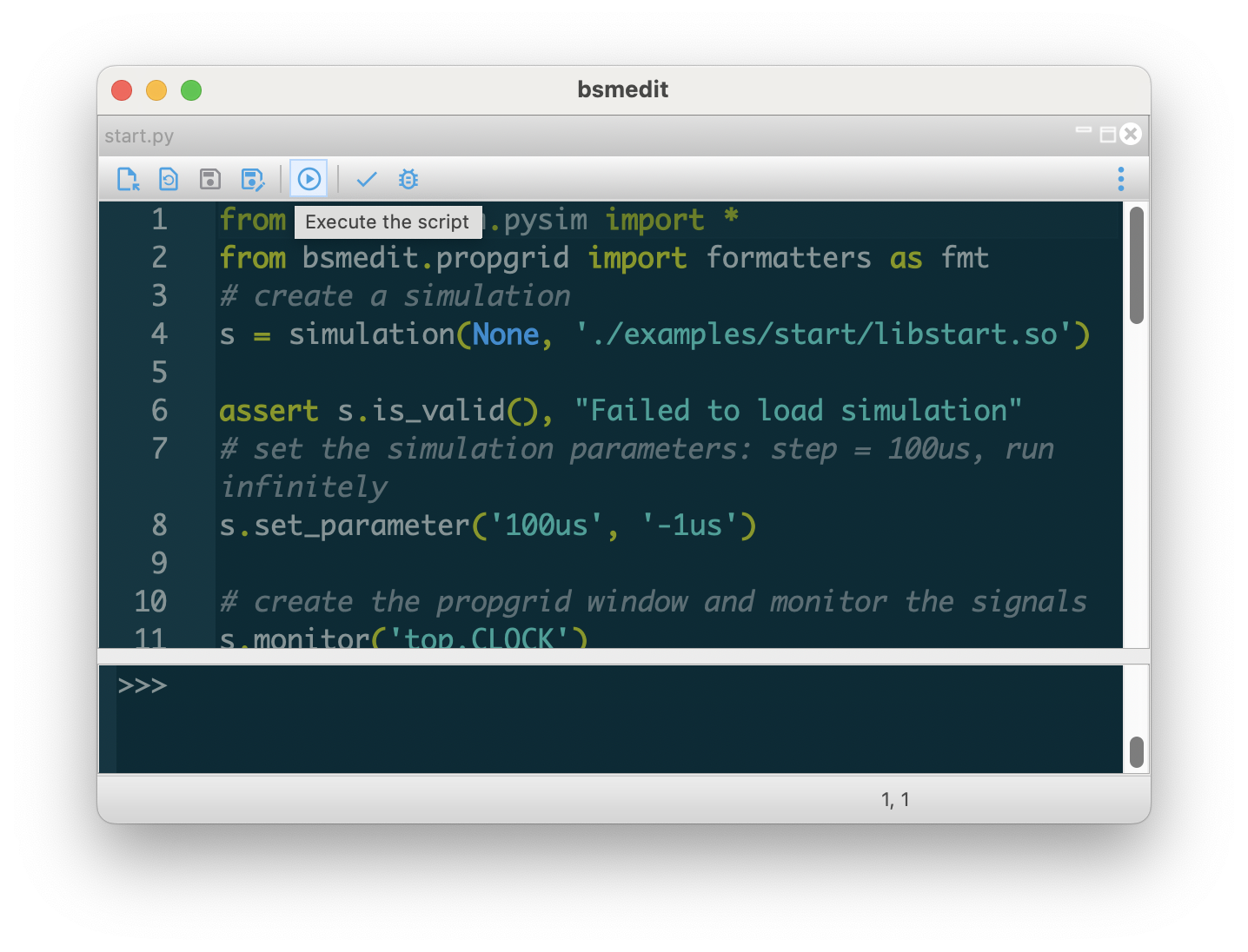
bsmedit will load the simulation, create a propgrid window, monitor the signals, and create a figure to plot the signals.

3 How it works

bsmedit was initially written in C++, which can be found here. It looks like an ideal choice since the simulation is also written in C/C++/SystemC. It supports multiple platforms (e.g., windows, linux), as the GUI is based on wxWidget.

It is highly extensible thanks to the plugin system. Actually most functions as you seen above were implemented with the plugin system. For example, one plugin is used to control the simulation (e.g., start, pause, stop, resume), which also supports breakpoints (e.g., pause the simulation when some conditions are satisfied; thus, you can check the status of your algorithm at that time.). One plugin is to plot the data captured from the simulation, which mimics some features from Matlab plot function: you can visualize the data in real-time and check its trend dynamically. One plugin adds some basic DSP functions (e.g., max, min, median, addition, subtraction, multiplication (dot product), square, square root, log/exp, sin/cos, acos/asin, tan, FFT etc.). It also had a console window so that you can run python command (e.g., to control the simulation)...

Following this way, we could build bsmedit block by block. At that time, I though it would work. However, such method has some significant drawbacks. One big problem is that we need to re-invert many many wheels. For example, after implement some functions, bsmedit also needs to wrap all these functions in python, so that you can call it in python script or in the console window. No need to say how tedious and error-prone such process is. How about adding a DSP function that does not exist in bsmedit (e.g., a moving average)? Basically, you will have to create a plugin project following the template, and write code to implement the actual processing. We try hard to make the interface as simple as possible; but it still requires some significant effort to make such plugin work. Furthermore, how about adding some features to the plot library? It will be a real nightmare to go through all the code to find the right position to add some code...

To solve these issues, from version 3, bsmedit is totally rewritten with python (wxPython for GUI). But, it does not mean you need to write your simulation in python. The simulation is still in C/C++/SystemC, and bsmedit will load and run the simulation as usual. Since it is in python, all functions can be directly called by python script and no need to wrap the interfaces any more. No need to provide a custom plot library, since you can just use the existing python libraries (e.g., matplotlib). No need to write many basic DSP function, which can be easily fulfilled with numpy or scipy...

3.1 Console window

In version 3, the python console window is replaced with a native interactive interpreter (wx.py.shell). It allows you to run arbitrary python command.

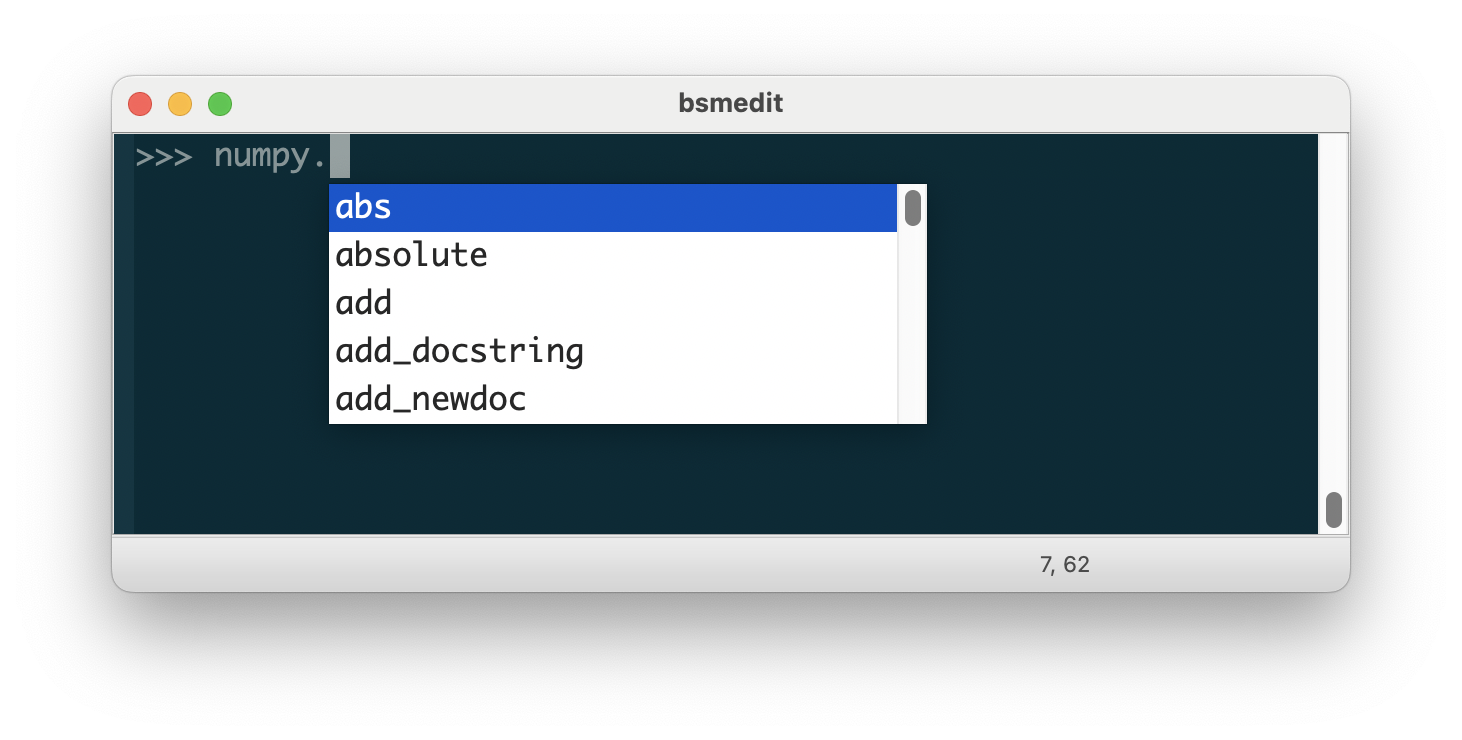
It is not fun to remember all the commands. When typing a '.', bsmedit will show an auto-complete list for you to select from, if there is any

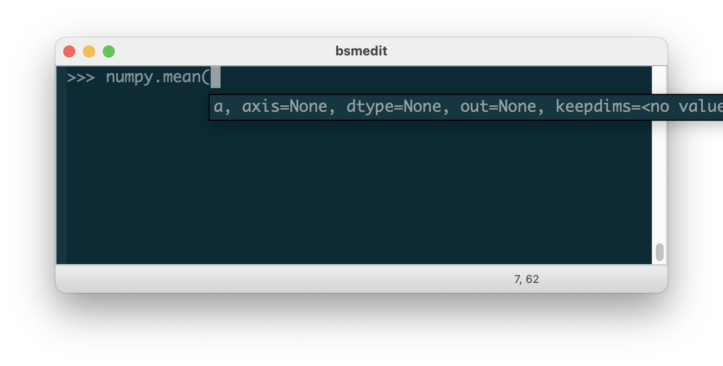
Similarly, it will also try to show the calltips of a function when it sees a '('

It also supports executing external command. The external command should be prepended by '!'. For example, to list the contents in the current folder by calling 'ls' command (see here for windows system)

>>> !ls

You can also pass arguments to the external command

>>> !ls -l

By default, when executing the external command, bsmedit will wait for it to finish, then show its output in the console window. Command can also be executed in background by appending a '&'. For example, the following command will open a gvim window and return (without '&', it will not return until the gvim window is closed)

>>> !gvim &

You can add an alias to an external command to save some typing. For example, the following command will add an alias ll

>>> alias ll ls -l

where the first parameter is the alias name (e.g., ll), and the remaining parameters are the destination (e.g. ls -l). Now, when the console sees input ll, it will automatically replace it with !ls -l, and execute it. If an alias definition does not include a destination, it will be deleted if exists. For example, the following code will delete the alias ll

>>> alias ll

There are some pre-defined commands (by wx.py.shell), which are frequently used. Thus, you still can used it even if these external commands are not installed.

>>> cd DIR # go the DIR folder
>>> pwd # show the current working directory
>>> ls # list the current working directory
>>> clear # clear the console window

It is also able to run the command silently by appending ';'. In other words, to execute the command without showing any output in the console window.

>>> # define a function foo
>>> def foo():
...    print('foo')
...    return 42
...
>>> # call a function with output
>>> a = foo()
foo
>>> # call a function silently
>>> a = foo();
>>>

One major constraint of version 3 is that it executes the command in the main GUI thread. Thus, if a dead loop is fed into the interpreter, it will never return and can not be interrupted, for example:

>>> while True:
...    pass

One reason we do not execute the command in a separate process or thread is that some command may create GUI window. If the GUI window is created in separate process/thread, it will potentially cause many problems and significantly increase the complexity to handle the GUI window. However, in bsmedit, most time-consuming task should be the simulation itself, not the command or processing. Thus, the console command should not occupy too much time to block the GUI updating.

3.2 Figure

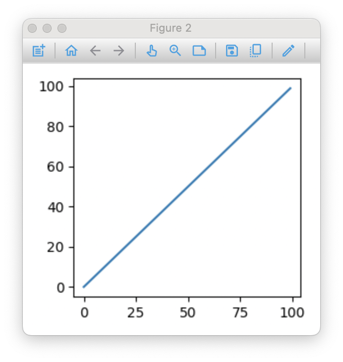
In version 3, the original plot library is discarded. Instead, we use matplotlib to visualize the data. By default, all the functions defined in matplotlib.pyplot are pre-loaded, so you can call them directly in the console window. The detailed description can be found here. To create a new figure and plot a straight line

>>> figure();
>>> plot(range(100))

and the figure will look like

Like Matlab, you can add label, legend, and grid

>>> xlabel('x')
>>> ylabel('y')
>>> grid(ls='dotted')
>>> legend(['line1'], loc='best')

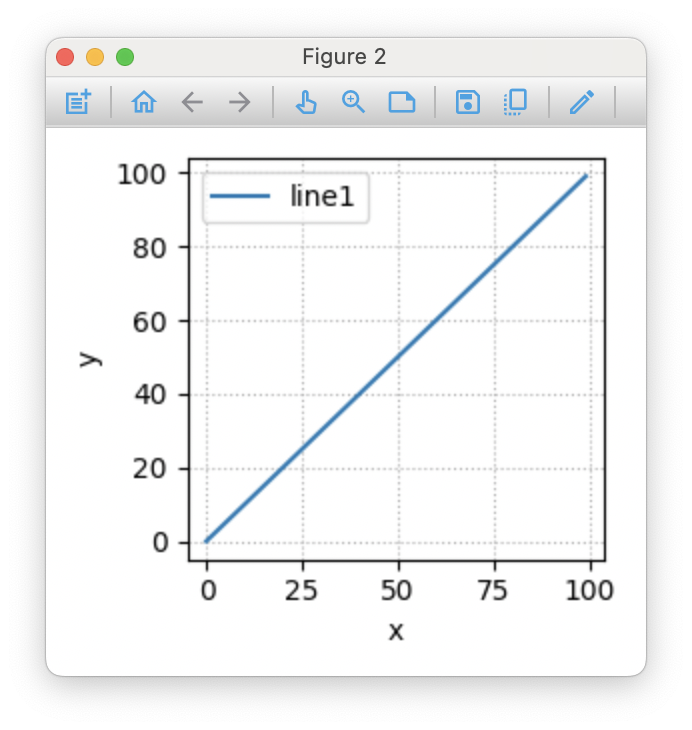
As shown above, the figure window has two sections: toolbar and plot. The buttons on the toolbar are (from left to right)

new figure: create an empty figure
home: it will bring the plot to the initial status (e.g., zoom and position)
back: go to the previous status if available
forward: go to the next status if available
move/pan: move the plot with the mouse
zoom: zoom in the plot by clicking, moving and releasing mouse, or with the mouse wheel. Double-click on the plot will bring the plot to the original view.
datatip: add datatip to the curve.

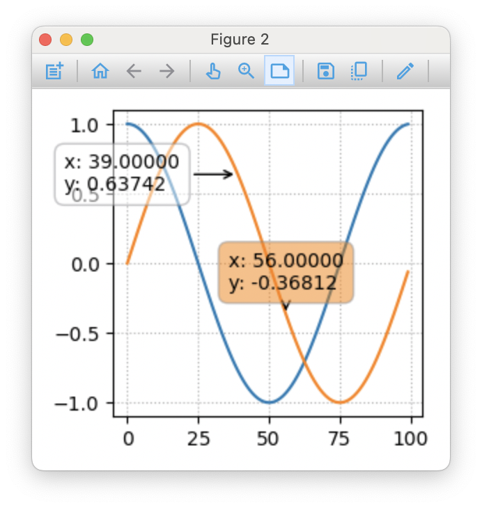
datatip can be activated by clicking on it and its background will be in orange. In this case, you can drag the datatip around to align it in different position.
save: export the plot (without the toolbar section) to a file (e.g., with format eps, ps, pgf, png, pdf, raw, rgba, svg ... )
copy: copy the plot (without toolbar section) to clipboard
edit: edit the plotted lines

The plot function will add the curve to the active figure window. Generally, the active figure window is the latest activated figure window. For example, you can click on a figure window to make it active. And it will keep active until you click on another figure window or create a new one. If you are not sure about the active figure window, you may click on it before calling any plot functions. For a figure with multiple subplots, click the one to activate it

The following command will activate the figure window with number 1 (its window name may look like "Figure 1")

>>> figure(1)

You can also get the handle of the current figure with

>>> # get a reference to the current figure
>>> gcf()
>>> # get the current axes on the current figure
>>> gca()

Refer to the Matplotlib doc for more details.

3.3 Simulation

One problem in version 2 is that the SystemC simulation runs in a thread, and it may crash, which may in turn crashes bsmedit. In version 3, the simulation runs in a separate process, which receives command from the main process (e.g., interactive interpreter), executes it and sends the response back. In this way, the simulation can gracefully exit without affecting the main process.

As you have seen above, bsmedit defines functions to control the simulation

Create a simulation.

s = simulation(num=None, filename=None, silent=False, create=True, activate=False)

where

num	the simulation id. If a simulation with num is found, its handler will be returned
filename	the simulation path
silent	False: open a file dialog to select a simulation if filename is not given True: do not show a file dialog
create	create a simulation if can not find a simulation
activate	activate the simulation window if it is True

If the function is executed successfully, it will return the handler to the simulation, which can be used to control the simulation or have access to its objects. For example

# create a simulation and load 'mysimulation.dll'
s = simulation(filename='./mysimulation.dll')
# return the handler of the simulation #1 if it is available
s = simulation(1)

Load the simulation.
```
s.load(filename=None)
```
where the parameter filename is the path to the simulation. If a simulation has already been loaded, load will unload it first.

If filename is None, a file-select dialog will be shown to select the simulation.

Set simulation parameters.

s.set_parameter(step=None,  total=None,  to=None,  more=None,  **kwargs)

where

step	the time duration of each step, e.g., "100us". The pre-defined time units include fs (femtosecond), ps (picosecond), ns (nanosecond), us (microsecond), ms (millisecond), and s (second).
total	the total simulation duration; -1 means to run infinitely.
to	pause simulation when simulation time reaches to (or total).
more	run simulation for additional time defined by more, then pause. If to is also defined, to has higher priority.

For example

# set the step to be 1000us, and run infinitely
s.set_parameter(step='1000us', total='-1')
# set the step to be 1000. Here unit is not given, so the current one will be used. The default unit is 'ns'
s.set_parameter(step='1000', total='-1')
# When 'run' the simulation, it will stop at 100ms
s.set_parameter(to='100ms')
# When 'run' the simulation, it will stop at 100ms from the current simulation time-stamp
s.set_parameter(more='100ms')

Run the simulation. There are several functions to start the simulation
```
# run the simulation for a single step with current settings (step, total)
s.step()
# run the simulation with the current settings (step, total)
s.run()
# run the simulation until 1ms
s.run(to='1ms')
# run the simulation for additional 1ms
s.run(more='1ms')
```
Sometime, you may want to wait until the simulation pauses. For example, you may want to check the signal value after the simulation has paused. There is a function to do that
```
s.wait_until_simulation_paused()
s.read('top.sig_sin')
```
It will return only if the simulation is valid and has paused (in this case, it will return True), or the simulation is invalid (return False). And the second line s.read will not be called until s.wait_until_simulation_paused has returned. You can also set the timeout. For example, the following command will wait for a maximum period of 10s
```
s.wait_until_simulation_paused(10)
```
Here 10s is the 'PC time', not the simulation time.
Pause the simulation.
```
s.pause()
```
It will pause the simulation, but not destroy it. In other words, you can resume the simulation by calling step or run mentioned above. To permanently destroy the simulation, you can call
```
s.stop()
```
Reset the simulation.
```
s.reset()
```
It will close the current simulation, and reload it. Thus, when it is executed successfully, the simulation time will be reset to 0.

Read signals. bsmedit defines function to have access to the signals in the simulation, for example

>>> # read a single signal
>>> s.read("top.sig_cos")
0.7958369046061

Besides calling the read function explicitly, you can also use a shortcut

>>> # same as the previous command
>>> s["top.sig_cos"]
0.7958369046061

You can also read multiple signals with one command. In this case, the return value will be a dict, whose key is the signal name.

>>> # read multiple signals
>>> s.read(['top.sig_cos', 'top.sig_sin'])
{'top.sig_sin': 0.60551104140799, 'top.sig_cos': 0.7958369046061}
>>> # equivalent to
>>> s[['top.sig_cos', 'top.sig_sin']]
{'top.sig_sin': 0.60551104140799, 'top.sig_cos': 0.7958369046061}
>>> # equivalent to
>>> s['top.sig_cos', 'top.sig_sin']
{'top.sig_sin': 0.60551104140799, 'top.sig_cos': 0.7958369046061}

For SystemC simulation, bsmedit supports the following data types. The right column shows the corresponding data type in python.

SystemC type	Python type
float, double	float
bool, char, unsigned char short, unsigned short int, unsigned int long, unsigned long long long, unsigned long long sc_logic, sc_bit	long
sc_lv, sc_bv sc_int, sc_uint sc_bigint, sc_biguint sc_fixed sc_fixed_fast sc_ufixed std::string³	string

And you can use the above function to read all the sc_signal, sc_out, sc_inout, and sc_in objects.

Write signals. To update the signal value, you can call
```
s.write(objects)
```
where objects is a dic with the signal name as its key. bsmedit supports writing all the sc_signal, sc_out, and sc_inout⁴.

Due to the two-step mechanism in SystemC, in most cases, the value will be updated after the next delta cycle. That is, if a read is called after write immediately, it may return the previous value.
```
>>> s.read('top.sig_steps')
256
>>> s.write({'top.sig_steps': 8192})
>>> s.read('top.sig_steps')
256
```
Like read, there is also a shortcut to write the signal
```
>>> # same as the command above
>>> s['top.sig_steps'] = 8192
```
Similarly, you can also write to multiple signals by calling write once
```
>>> # write multiple signals
>>> s.write({'top.sig_steps': 8192, 'top.sig_sin': 0.1})
>>> # same as the command above
>>> s[['top.sig_steps', 'top.sig_sin']] = [8192, 0.1]
>>> # or
>>> s['top.sig_steps', 'top.sig_sin'] = [8192, 0.1]
```

Dump signal to numpy array. For example, by calling the following command

>>> s.trace_buf('top.sig_cos', size=10)

bsmedit will dump the values of top.sig_cos to a numpy array, so you can manipulate it easily. In the above example, the buffer size is 10. If the size is not set, the default size will be 256. Then, the buffer can be accessed by

>>> buf = s.read_buf('top.sig_cos')
>>> type(buf)
<type 'numpy.ndarray'>

The buffer will be filled with the most recent 10 samples, where $\textrm{buf}[9]$ is current one and $\textrm{buf}[0]$ is the oldest. One thing we haven't talked about is how these samples are saved. By default, a samples is saved to the buffer only when the value is changed, for example, either rising edge or falling edge. For rising edge, it means the current value is larger than the last value; while for falling edge, the current value is smaller than the last value.

In some application, it may work well. For example, if the output of the signal is shown as the following figure,

then at time $t=9$, the buffer will be $[0, 1, 0, 1, 0, 1, 0, 1, 0, 1]$, as expected. However, if the signal output is as the one shown in the figure below. The data in buffer may look like $[x, x, x, x, x, x, x, 0, 1, 0]$, where $x$ is the value either from the buffer initialization or previous samples, rather than $[0, 1, 0, 0, 0, 0, 0, 0, 0, 0]$. The result is not surprising since the simulation will only push the data to the buffer whenever the data is changed. However, the value does not changed within $t=[2,3,...10]$

You may want to only dump the data at the rising (or falling) edge. In this case, replace the above trace_buf with

>>> s.trace_buf('top.sig_cos', size=10, trigger='pos')

Then the buffer will only be filled when the signal value is increased (compared to the last value). In particular, for the above figure, at $t=9$, the buffer will be $[x,x,x,x,x,x,x,x,x,1]$.

Similarly, you can also dump the signal only at its falling edge

>>> s.trace_buf('top.sig_cos', size=10, trigger='neg')

In some case, you may want to dump the signal at a fixed sampling clock. How could we do that with bsmedit? Actually it is also straightforward. What we talked so far is to only use the signal itself to dump the value. bsmedit also provide a way to trigger the dumpling with a valid signal; that is, the dumping can be triggered by the rising and/or falling edge of a valid signal

>>> s.trace_buf('top.sig_cos', size=10, valid='top.CLOCK', trigger='pos')

It tells bsmedit to allocate a buffer with size 10 and dump the value to it at each rising edge of the signal top.CLOCK.

For example, for the signals shown in above figure, at $t=9$, the buffer will be $[2, 3, 2, 2, 2, 2, 2, 2, 2, 2]$.

Since the value is dumped to a numpy, you can process the data with all the functions available (e.g., signal processing with scipy.signal or plot with matplotlib) . And bsmedit also provides a function to plot the trace dynamically

plot_trace(x=None, y=None, relim=True, *args, **kwargs)

where

x	signal name for x-axis (e.g., 'top.sig_cos')
y	signal name for y-axis (e.g., 'top.sig_sin')
relim	automatically calculate the x & y limits
args, *kwargs	additional arguments to Matplotlib plot function

For example,

>>> plot_trace('top.sig_cos', 'top.sig_sin')

Then when you run the simulation, the plot will be automatically updated accordingly

Dump signal to a file.

s.trace_file(name='',  filename='',  fmt='bsm',  valid=None,  trigger='posneg',  **kwargs)

where

dump object values to a file

        name:
            register name
        filename:
            trace filename
        fmt:
            'bsm': only output the register value, one per line (Default)
            'vcd': output the SystemC VCD format data
        valid:
            the trigger signal. If it is none, the write-operation will be
            triggered by the register itself
        trigger:
            'posneg': trigger on both rising and falling edges
            'pos': trigger on rising edge
            'neg': trigger on falling edge
            'none': no triggering

For example, to trace the signal top.sig_sin in to file top.sig_sin.bsm

s.trace_file(name='top.sig_sin')

Monitor signal in a propgrid window.
```
s.monitor(objects, grid=None, index=-1, style='Text', **kwargs)
```
If progprid is None and no propgrid window (see Sec. 3.4 for details) has been created, bsmedit will create one and add the signal to it. For example, the following line will monitor signal top.sig_double in the active propgrid
```
s.monitor('top.sig_double')
```
Breakpoints. With the simulation control functions mentioned above, you can easily pause the simulation at particular simulation time. However, in some cases, you may want to pause the simulation when some conditions meet. The breakpoint is here to rescue. To set a breakpoint,
```
s.add_breakpoint(name, condition=None, hitcount=None)
```
where

name the signal name (e.g., top.sig_cos)

condition the breakpoint condition (optional)

hitcount the hit count condition (optional)

bsmedit will check the breakpoint at each SystemC delta cycle. Once the breakpoint condition is true (or signal value is changed if condition is None), it will pause the simulation.

The breakpoint condition can be any valid python statement, for example
```
s.add_breakpoint('top.sig_cos', '$>=0.9', None)
```
Here $ will be replaced with the signal value before checking breakpoint condition. Then, bsmedit will pause the simulation whenever its value is larger than 0.9.

You can also set the hit count, for example,
```
s.add_breakpoint('top.sig_cos', '$>=0.9', '#==4')
```
Again, # will be replaced with the hit count. The breakpoint will only be triggered if the breakpoint condition has been true for at least 4 delta cycles. In other words, the breakpoint has been hit for at least 4 times.

You can also retrieve all the breakpoints by
```
>>> s.get_breakpoint()
[['top.sig_cos', None, None]]
```
To delete a breakpoint,
```
s.del_breakpoint('top.sig_cos', None, None)
```
Here you also need to provide the full definition of the breakpoint, since multiple breakpoints may share the same signal, and/or breakpoint condition, and/or hit-count condition.

The breakpoint here is different from the one when you debug the C/C++/SystemC source code. For example, if you add the same breakpoint 5 times, it will not be cleared until you delete all 5 instances.
```
>>> bp = ['top.sig_cos', None, None]
>>> # add one
>>> s.add_breakpoint(*bp)
>>> s.get_breakpoint()
[['top.sig_cos', None, None]]
>>> # add it again
>>> s.add_breakpoint(*bp)
>>> s.get_breakpoint()
[['top.sig_cos', None, None], ['top.sig_cos', None, None]]
>>> # delete one
>>> s.del_breakpoint(*bp)
>>> s.get_breakpoint()
[['top.sig_cos', None, None]]
```
After all these steps, there is still a breakpoint. You can use the get_breakpoint command to confirm. Thus, it will still pause the simulation once its condition is met. At first sight, such behavior seems annoying, useless and confusing (as in most debugger, you may only set one breakpoint at each single line). However, since a signal can be added to propgrid window multiple times, and you may enable the breakpoint by clicking the radio button (as shown in the section below), it may cause confusion if bsmedit only keeps one instance of each distinct breakpoint. That is, bsmedit may have deleted the breakpoint, but the propgrid window shows it is still valid. So each add_breakpoint needs to be explicitly canceled by one del_breakpoint.
Multiple simulations. Version 2 only supports running one simulation. So to run multiple simulations, you need to run multiple bsmedit. It is not very convenient to compare the results from multiple simulations. For example, it is impossible to show results from different simulations in a single plot (actually you may be able to do so by dumping the data to files). In version 3, bsmedit supports running multiple simulations simultaneously (each in its separate process). In this way, you can even run the same simulation in multiple processes; and each one is independent to the others. For example, the following commands will run the same simulation core in two separate processes. With that, you can configure the simulation differently to compare the result.
```
>>> s1 = simulation(None, './examples/start.dll')
>>> s2 = simulation(None, './examples/start.dll')
```
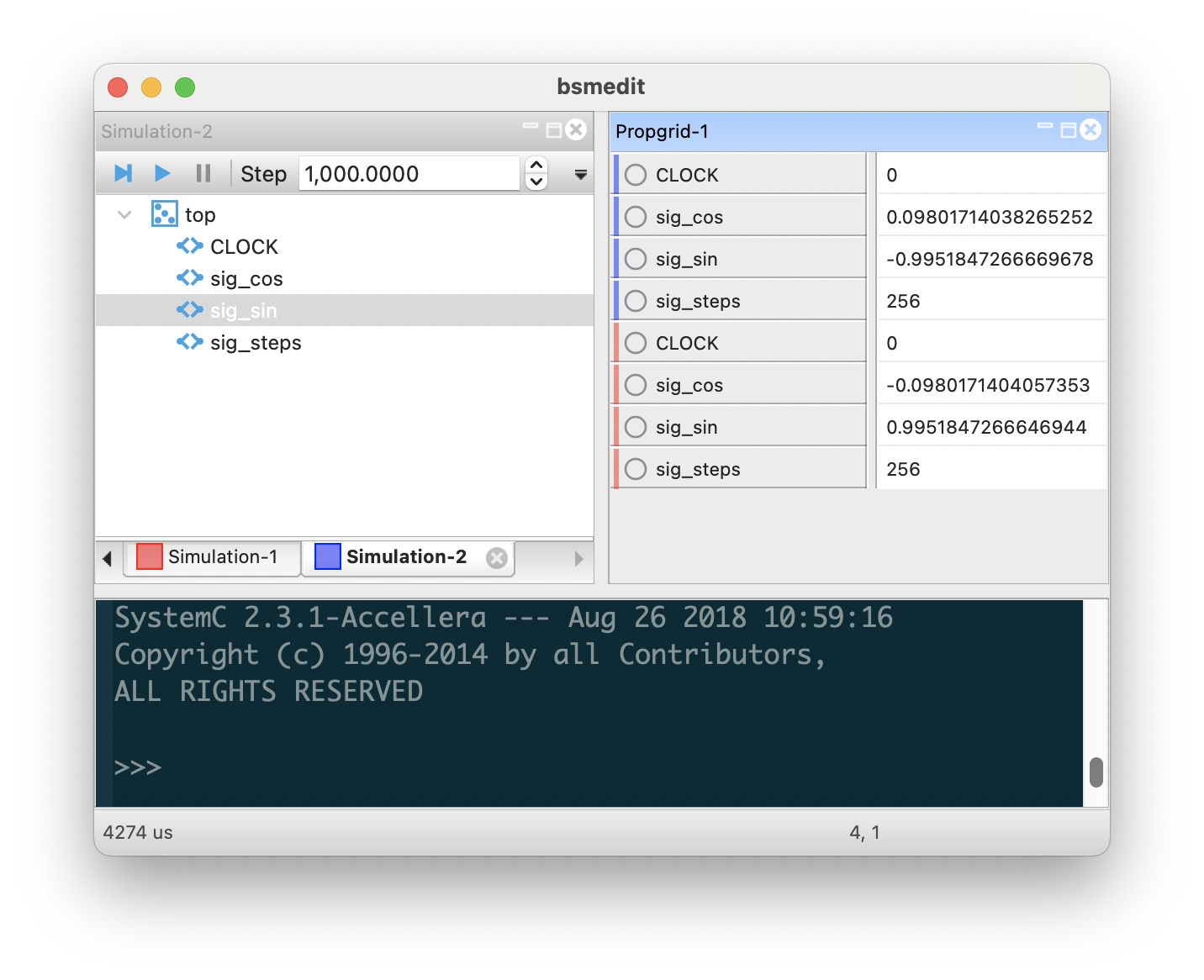
To differentiate the simulations, each simulation will automatically be assigned an id (e.g., 1,2,3...).

With that id, you can retrieve the simulation handler later by
```
>>> s1 = simulation(1)
```
which will return the handler to Simulation-1.

3.4 Propgrid window

As shown above, each signal in propgrid has two sections: label and value.

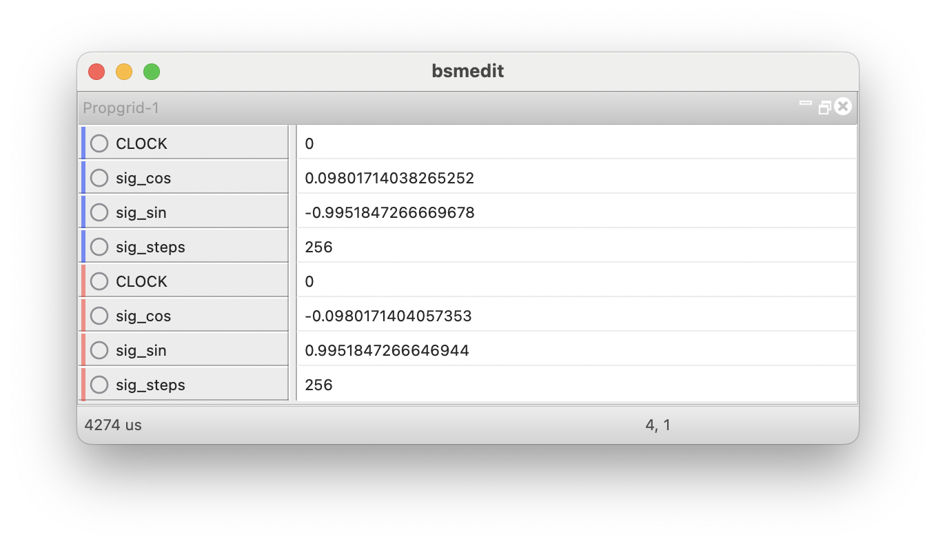
Order the signals. In general, the signals are shown in a propgrid window according to the order they are added. However, you can easily re-order the signals. There are two ways to do so

drag the signal to the new destination
select the signal (the selected signal will be highlighted)
- right click on the signal to show the context menu
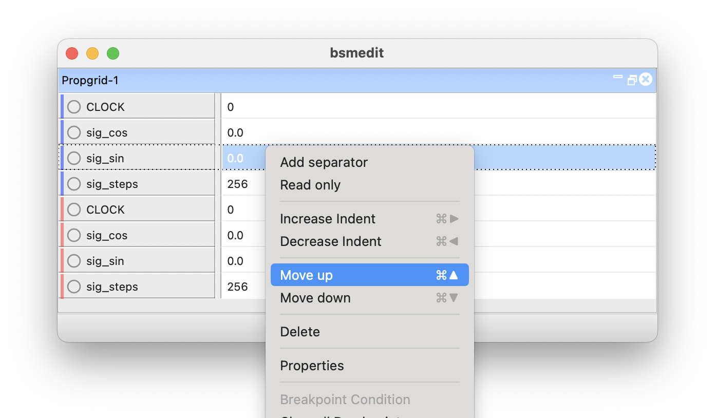
- or press Ctrl/Cmd+Up/Ctrl/Cmd+Down to move the signals up/down.

Group multiple signals together. Right click on a signal to show the context menu, and click the Increase Indent

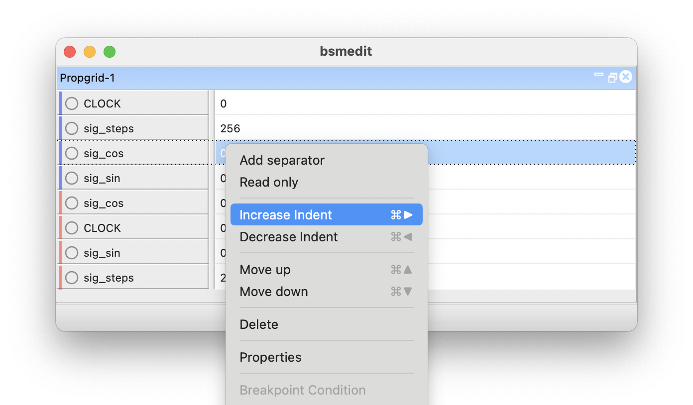
Then bsmedit will increase the indent of the signal, and the signal will effectively becomes the child of the previous signal (with smaller indent level).

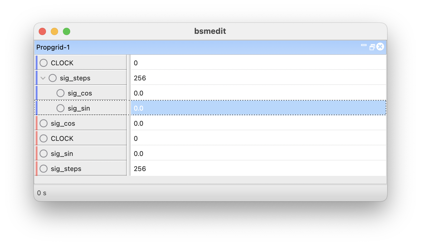
You can also use script to change the indent level

>>> # get the propgrid window with id=1
>>> g = propgrid(1)
>>> # get the handle of the property (assume it has already been added to the
>>> # propgrid window. Since the properties in each propgrid window may monitor
>>> # signals from multiple simulations, and they may have same name, here the
>>> # signal name is the global name. In other words, the original signal name is
>>> # prepended with its simulation id.
>>> p = g.Get("1.top.sig_sin")
>>> # to increase the indent by one level
>>> p.SetIndent(p.GetIndent()+1)
>>> # to decrease the indent by one level; the minimal indent level is 0
>>> p.SetIndent(p.GetIndent()-1)

You can click the +/- button to show/hide the children.

>>> p = grid.Get("1.top.sig_steps")
>>> # show the children signals
>>> p.SetExpand(True)
>>> # hide the children signals
>>> p.SetExpand(False)

Use the control to set the signal. As you see before, each signal in the propgrid has two sections: name and value. The value section shows its current value. When click on the value section, if the signal is writable, the signal will be in edit mode; by default, an editbox will be shown so that you can type the value. By typing Enter after modifying the value, bsmedit will send the change to the simulation.

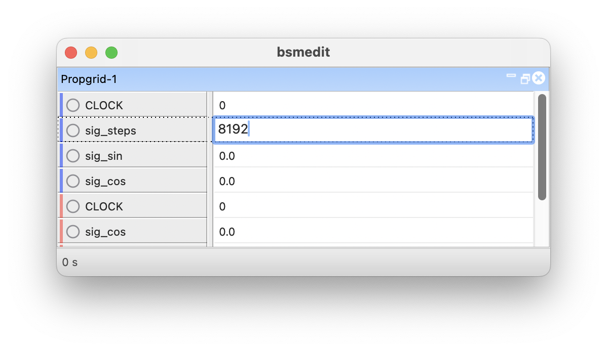
Besides the editbox, the following types of controls can be used to update the signal values

Combobox

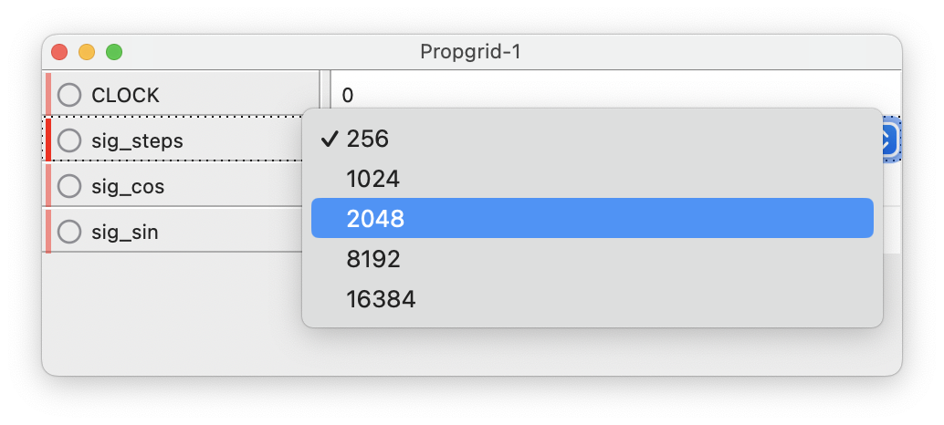
You can right click on the signal and select 'Properties' from the context menu to change the window type in edit mode. Besides that, it can also be changed by python script:
```
p = g.Get('1.top.sig_steps')
p.SetControlStyle('Choice', choice=[256, 1024, 2048, 8192, 16384])
```

Slider

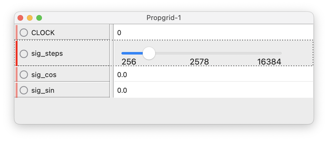
p.SetControlStyle('Slider', min_value=256, max_value=16384)

Spin

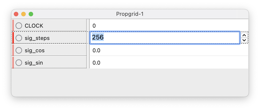
p.SetControlStyle('Spin', min_value=256, max_value=16384)

Checkbox

p = g.Get('1.top.sig_sc_bit')
p.SetControlStyle('CheckBox')

Radio box

p = g.Get('1.top.sig_logic')
p.SetControlStyle('RadioBox', choice=['1', '0', 'Z', 'X'])

Color picker
Select File/Folder button

As shown above, you can set the breakpoint with script. You can also set the breakpoint in propgrid window by clicking the radio button next to the signal name:

bsmedit will check the breakpoint at each SystemC delta cycle. Once the condition is true, it will pause the simulation. The breakpoint can also be enabled by python script:

p.SetChecked(True)

Then, if you run the simulation, it will be paused once the signal value is changed or the simulation time is reached. You can also set the breakpoint conditions here. Right click on the signal and click 'Breakpoint Condition' (the menu item is not clickable unless the radio button is checked)

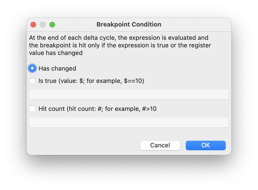
When the "Is true" radio button is checked, the condition editbox will be enabled for input. For example, "$>0.1" will pause the simulation when the signal value is greater than 0.1, where "$" will be replaced by the signal value. Breakpoint condition can also be set by

p.SetBpCondition('$>0.1','')

When hit count is set (e.g. #==4), the breakpoint will only be triggered if the breakpoint condition has be met for certain amount of delta cycles (e.g., 4 delta cycles).

p.SetBpCondition('$>0.1','#==4')

3.5 SystemC Simulation

From version 3, bsmedit supports SystemC 2.3. Once a simulation is loaded, bsmedit will have access to the following data types

bool
float, double
char, unsigned char
short, unsigned short
int, unsigned int
long, unsigned long
long long, unsigned long long
sc_logic, sc_bit
sc_lv, sc_bv
sc_int, sc_uint
sc_bigint, sc_biguint
sc_fixed
sc_fixed_fast
sc_ufixed
std::string

And you can use the above function to read/write all the sc_signal/sc_out/sc_inout objects, and read all the sc_in objects.

To make bsmedit work, the simulation needs to implement and export some interfaces. bsm.h/cpp is the bridge between bsmedit and SystemC simulation. It implements the interfaces such that bsmedit can have access to all the objects and also control the simulation.

create the top level module

void bsm_sim_top(sim_context *context);

It is a first function bsmedit will call to create a simulation, where sim_context is a struct to return simulation information to bsmedit. It is defined by the macro "BSMEDIT_IMPLEMENT_MODULE"

typedef struct sim_context {
    char version[MAX_NAME_LEN];
    char copyright[MAX_NAME_LEN];
} sim_context;

#define BSMEDIT_IMPLEMENT_MODULE(T, name) extern bsm_sim_context* g_sim;\
extern "C" {\
    BSMEDIT_EXPORT void bsm_sim_top(sim_context *context) {\
        g_sim = new bsm_sim_context_impl(new T(name));\
        snprintf(context->copyright, MAX_NAME_LEN, "%s", g_sim->sc_copyright());\
        snprintf(context->version, MAX_NAME_LEN, "%s", g_sim->sc_version());\
    }\
}

bsm_sim_top creates the simulation context (i.e., g_sim). Then, bsmedit can control the simulation through all the other interfaces defined in bsm.h/cpp with that handler.

3.5.1 xsc_property

With SystemC's sc_signal, it is very easy to simulate a register in simulation. For example, you can configure the simulation by changing the values of some sc_signal without updating and re-compiling the source code. However, sometime you (the simulation) may want to know when the configuration is updated. For example, the simulation may want to log the configuration value once it is changed. Thus we derive the xsc_property from sc_signal.

Its usage is almost exactly same as sc_signal. It supports all the data type supported by sc_signal.

class MyModule:public sc_module {
public:
    MyModule(sc_module_name name_):
            tx_module(name_)
            ,xsc_prop_double("xsc_prop_double", this, xsc_callback_fun) {
        //set the value and don't call the callback function
    }
    xsc_property<double> xsc_prop_double;
    static void xsc_callback_fun(sc_module* pThis, double value);
};

In this example, we define a double type xsc_property. During its initialization, three parameters are passed into its constructor function:

its name derived from sc_signal,
the pointer to the current sc_module,
the pointer to a static function.

Now, when bsmedit sends the following command to the simulation (here assume the name/path of the xsc_property is "top.mymodule.xsc_prop_double")

>>> # s is the simulation handle
>>> s.write("top.mymodule.xsc_prop_double", 1.0)

The callback function xsc_callback_fun will be called, where its first parameter will be the pointer of the sc_module that defined the xsc_property, and the second parameter will be '1.0'.

The callback function should have the following format

typedef void(*xsc_callback)(sc_module* pThis, T value);

Sometime, you may want to only execute the callback function when it is updated externally (e.g., by bsmedit), but not internally (e.g., by the simulation itself). In this case, in your simulation code (e.g., C++), you may

xsc_prop_double.write_nc(128.0);

In this way, xsc_property behaves exactly same as sc_signal, and no callback function will be called.

3.5.2 xsc_array

xsc_array is a natural extension of xsc_property. It is actually an array of the xsc_property

class MyModule:public sc_module {
public:
     MyModule(sc_module_name name_)
     : sc_module(name_)
     , xscarray_int("xsc_array_int") {
         // set the value
         xsc_array_int[0] = 1;
         xsc_array_int[1].write(1);
         // get the value
         int a = xsc_array_int[0];
         int b = xsc_array_int[1].read();
     }
     xsc_array<int, 5> xsc_array_int;
  };

The above example show to use xsc_array in a sc_module. It define an integer xsc_array with size 5. In the module's constructor, the xsc_arrary is initialized with name xsc_array_int. And it also shows the basic usage of xsc_array. Basically, it behaves as an array of xsc_property. You can use the [i] to have access to the $i$th item in the array.

Same as xsc_property, xsc_array also supports a callback function. For example

class MyModule:public sc_module {
public:
     MyModule(sc_module_name name_)
     : sc_module(name_)
     , xscarray_int("xsc_array_int", this, xsc_callback_fun) {
     }
     xsc_array<int, 5> xsc_array_int;
     static void xsc_callback_fun(sc_module* pThis, double value);
  };

In bsmedit, the item of the array can be accessed by its name. For example, if in the simulation, the above MyModule is a top level module with name "top", the first item of the xsc_array_int can be accessed by

>>> s.read('top.xsc_array_int[0]')

3.6 C/C++ Simulation

For SystemC simulation, bsmedit pre-defines some interfaces, which are implemented by each simulation. Then, bsmedit retrieves these interfaces to control the simulation (e.g., via ctypes). Same idea can be extended to any C/C++ simulation.

For example, assume your C/C++ code generates a 2D wave (e.g., received from a sensor). You may define the interface as

#ifndef _WAVE_H_
#define _WAVE_H_
typedef int (*pyCallback)(int);
typedef struct wave_frame {
    int rows;
    int cols;
    float* frame;
    int max_frame_len;
    pyCallback callback;
} wave_frame;

void get_frame(wave_frame* frame);
void get_frames(wave_frame* frame);
#endif  // _WAVE_H_

The wave_frame struct defines the data format sent to bsmedit:

the values and its dimension;
the callback to notify bsmedit that new data is arrived.

get_frame function is used to send one frame of data to bsmedit; and get_frames is to retrieve all the frames (e.g., imaging the C/C++ code is keeping receiving data from the sensor). For this demo, we simply generate a 2D sine wave

#include <math.h>
#include <stdio.h>
#include <unistd.h>
extern "C" {
#include "waves.h"
}

void get_frame(wave_frame* frame) {
    static float initial_phase = 0;
    initial_phase += 2.*M_PI/100.0;
    if (initial_phase > 2.*M_PI)
        initial_phase -= 2.*M_PI;
    frame->rows = 30;
    frame->cols = 30;
    if (frame->max_frame_len < frame->rows*frame->cols)
        return;
    for (int i=0; i < 30; i++) {
        for (int j=0; j < 30; j++) {
            frame->frame[i*30+j] = cos(2*M_PI*i/30+initial_phase)*
                                   sin(2*M_PI*j/30+initial_phase);
        }
    }
}

void get_frames(wave_frame* frame) {
    while (1) {
        get_frame(frame);
        if (frame->callback) {
            if (!frame->callback(0)) {
                break;
            }
        }
        usleep(100000);
    }
}

And the makefile may look like

CC = g++
CFLAGS = -Wall -fexceptions -g -W -fPIC -DPURIFY -D_USRDLL

DEPS = waves.h
ODIR=obj
OBJ = main.o
OBJS = $(patsubst %,$(ODIR)/%,$(OBJ))

libwaves: $(OBJS)
    $(CC) -shared  $^ -o $@.so

$(ODIR)/%.o: %.c $(DEPS)
    $(CC) $(CFLAGS) -c $< -o $@

$(OBJS): | $(ODIR)

$(ODIR):
    mkdir -p $(ODIR)

.PHONY: clean

clean:
    rm -f $(ODIR)/*.o *.so
    rm -r $(ODIR)

To generate the library

$ make

Now the library is ready, let's start to build the python interface so that it can communicate with bsmedit. One way is to use ctypes directly.

Import the ctypes package
```
>>> from ctypes import *
```

Create the corresponding wave_frame structure in python

>>> class wave_frame(Structure):
...     SIM_CALLBACK = CFUNCTYPE(c_int, c_int)
...     _fields_ = [('rows', c_int),
...                 ('cols', c_int),
...                 ('frame', POINTER(c_float)),
...                 ('max_frame_len', c_int),
...                 ('callback', SIM_CALLBACK),
...                ]

Load the library built above

>>> dll = cdll.LoadLibrary('libwaves.so')

Retrieve the interface, and set the return and argument types accordingly

>>> get_frame = dll.get_frame
>>> get_frame.argtypes = [POINTER(wave_frame)]
>>> get_frame.restype = None

Call the interface to get the data dimension, which is done by calling get_frame without allocating data memory
```
>>> frame = wave_frame()
>>> get_frame(frame)
```

Allocate memory

>>> frame.max_frame_len = frame.rows*frame.cols
>>> frame_array = np.zeros(frame.max_frame_len).astype(np.float32)
>>> frame.frame = frame_array.ctypes.data_as(POINTER(c_float))

Get the wave
```
>>> get_frame(frame)
```

Plot with matplotlib

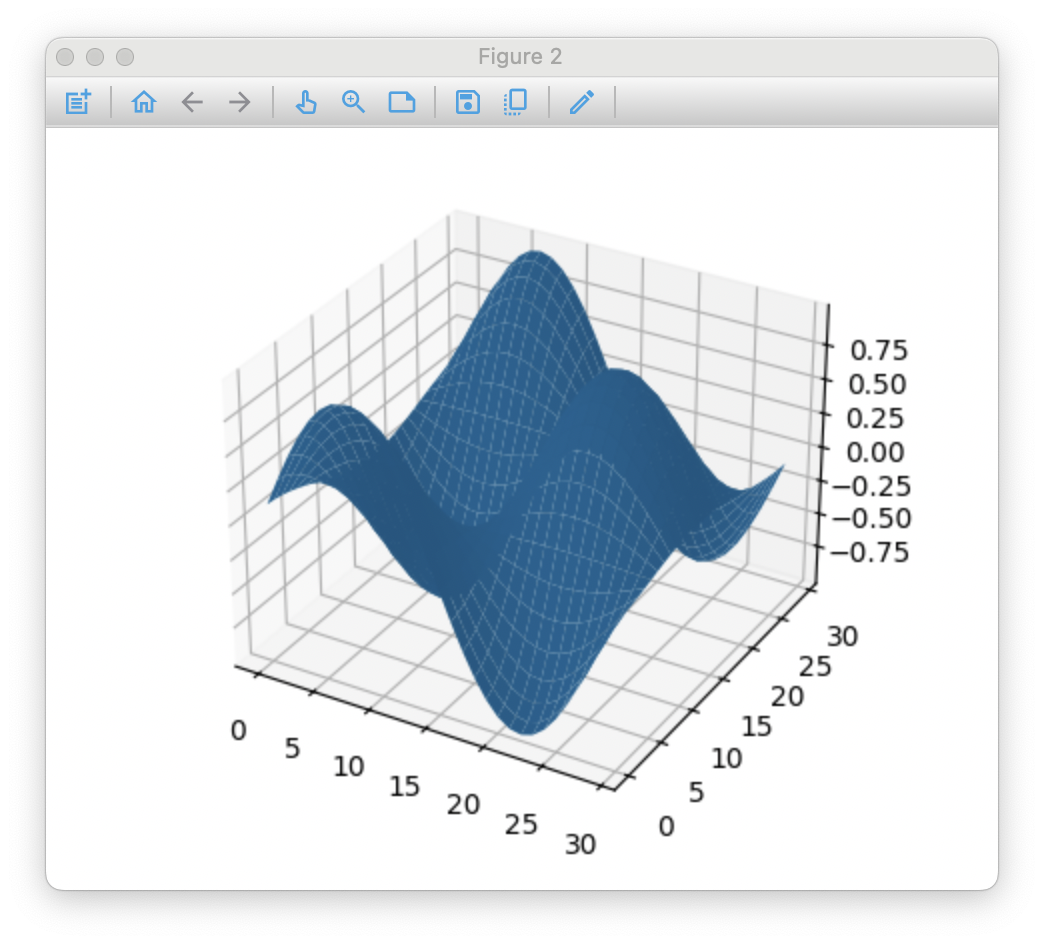
>>> x = np.meshgrid(np.arange(frame.rows), np.arange(frame.cols))
>>> fig = figure()
>>> ax = fig.add_subplot(projection='3d')
>>> ax.plot_surface(x[0], x[1], frame_array.reshape(frame.rows, frame.cols))

It is very flexible to build the python interfaces with ctypes directly. However, it is also tedious and error prone, especially when there are a lot of interfaces or the interfaces may change frequently. bsmedit provides an alternative way to automatically generate python interfaces from the header file, that is

bsmedit.bsm.csim.init_dll(dll, header)

where dll is the compiled library, and header is the corresponding header files, which defines all the interfaces. The function will return the python wrapper. Thus, the above example can be achieved by

>>> import bsmedit.bsm.csim as csim
>>> sim = csim.init_dll('./libwaves.so', './waves.h')
>>> f = sim.wave_frame()
>>> sim.get_frame(f)
>>> f.max_frame_len = f.rows*f.cols
>>> frame = np.zeros(f.max_frame_len).astype(np.float32)
>>> f.frame = frame.ctypes.data_as(POINTER(c_float))
>>> sim.get_frame(f)

The nice thing is that whenever the interfaces in header file (i.e., waves.h) is updated, just call csim.init_dll again (e.g., restart simulation), which will return the updated interface.

bsmedit also provides a class to to show the 3D image easily in python; the full example can be found here. Run the following command to show wave in bsmedit

$ bsmedit -i -p examples/waves waves

4 Misc.

4.1 VCD/CSV/Mat/ULog

When bsmplot is installed, bsmedit will also be able to visualize VCD/CSV//Mat/ULog time series. For example, ULog is the file format used in PX4 for message logging. The ulog plugin is to load and visualize the ulog messages. When open a ulog file (menu->open->ulog file), bsmedit will create a panel to show its content. Different types of message are shown in different tab.

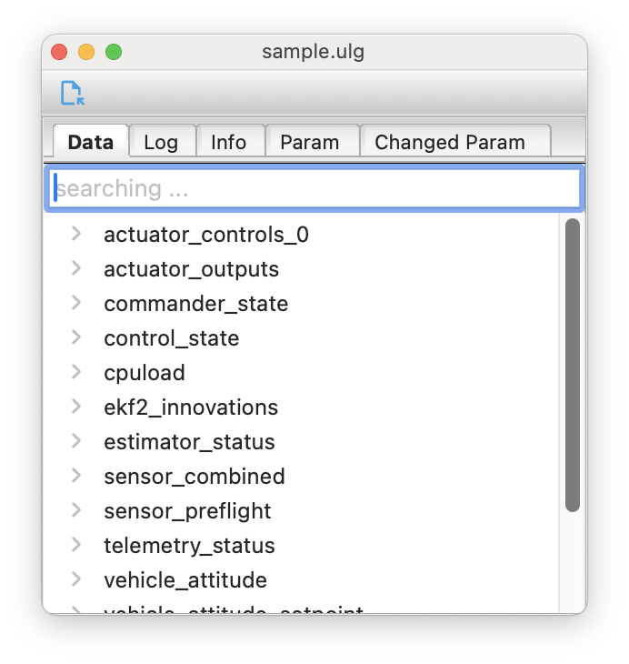
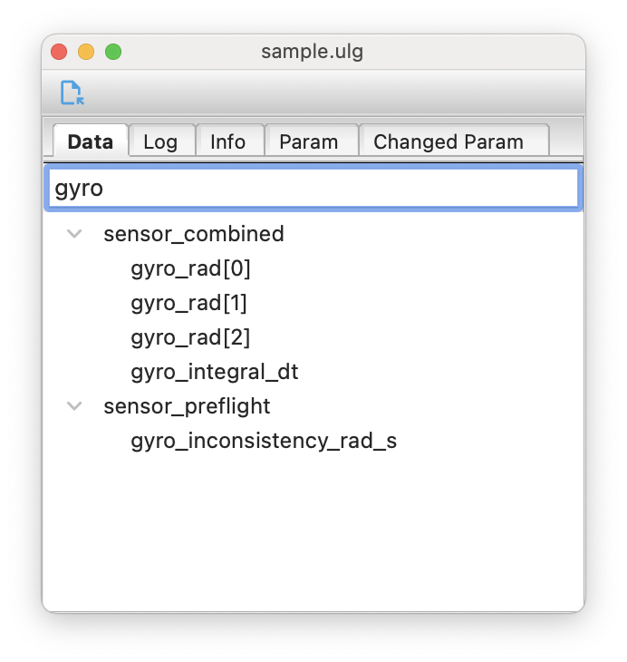
For a ulog file that has many messages, you can use the searching box to filter messages.

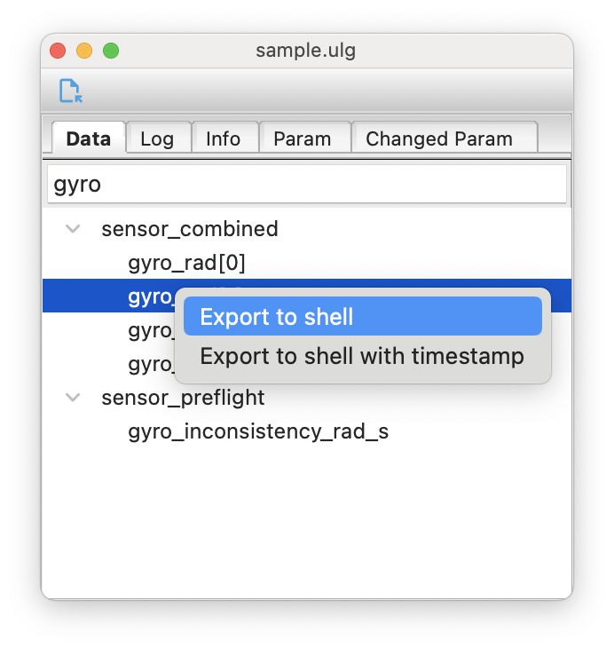
You can also export the data to the terminal by right click on it

To visualize the data, you can either

double click on the data, and it will on the current figure (create one automatically if no figure exists)
drag the data to some figure

Here we slightly abuse the notation simulation. It may be indicated as either the binary from the simulation project or the simulation instance in bsmedit. ↩

Sometimes they will be referred as objects (as they are all derived from sc_object) or signals (as sc_signal is the most common object to control the simulation). We will use both interchangeably. ↩

name	the signal name (e.g., top.sig_cos)
condition	the breakpoint condition (optional)
hitcount	the hit count condition (optional)